In strategy/management research, we always need to compile the regression results into the publishable format and sometimes plot the moderating effects. Thus, I developed this “regrrr” package to help do the job.

Here is the quickstart guide.

Installation

To install from CRAN:

install.packages("regrrr")
library(regrrr)

You can also use devtools to install the latest development version:

devtools::install_github("raykyang/regrrr")
library(regrrr)

Examples

compile the correlation table

library(regrrr)

## Registered S3 methods overwritten by 'tibble':
##   method     from  
##   format.tbl pillar
##   print.tbl  pillar

data(mtcars)
m0 <- lm(mpg ~ vs + carb + hp + wt, data = mtcars)
m1 <- update(m0, . ~ . + wt * hp)
m2 <- update(m1, . ~ . + wt * vs)
cor.table(data = m2$model)

##          Mean  S.D.     1     2    3    4    5
## 1.mpg   20.09  6.03  1.00                     
## 2.vs     0.44  0.50  0.66  1.00               
## 3.carb   2.81  1.62 -0.55 -0.57 1.00          
## 4.hp   146.69 68.56 -0.78 -0.72 0.75 1.00     
## 5.wt     3.22  0.98 -0.87 -0.55 0.43 0.66 1.00

compile the regression table

regression_table <- rbind(
combine_long_tab(to_long_tab(summary(m0)$coef),
                 to_long_tab(summary(m1)$coef),
                 to_long_tab(summary(m2)$coef)),
compare_models(m0, m1, m2))
rownames(regression_table) <- NULL
print(regression_table)

##        Variables   Model 0   Model 1   Model 2
## 1    (Intercept) 35.435*** 48.157*** 46.698***
## 2                  (2.503)   (4.097)   (9.272)
## 3             vs     1.353     1.077     2.171
## 4                  (1.382)   (1.152)   (6.320)
## 5           carb    -0.057    -0.043    -0.009
## 6                  (0.449)   (0.374)   (0.426)
## 7             hp   -0.024† -0.113***   -0.107*
## 8                  (0.014)   (0.027)   (0.044)
## 9             wt -3.792*** -8.071***   -7.594*
## 10                 (0.658)   (1.307)   (3.016)
## 11         hp:wt             0.027**    0.025†
## 12                           (0.008)   (0.015)
## 13         vs:wt                        -0.367
## 14                                     (2.081)
## 15     R_squared     0.833     0.889     0.889
## 16 Adj_R_squared     0.808     0.867     0.862
## 17       Delta_F            12.517**     0.031

plot the moderating effect

plot_effect(reg.coef = summary(m2)$coefficients, data = mtcars, model = m2,
            x_var.name = "wt", y_var.name = "mpg", moderator.name = "hp",
            confidence_interval = TRUE,  CI_Ribbon = FALSE, 
            xlab = "Weight", ylab = "MPG", moderator.lab = "Horsepower") +
ggplot2::theme(text=ggplot2::element_text(family="Times New Roman", size = 16))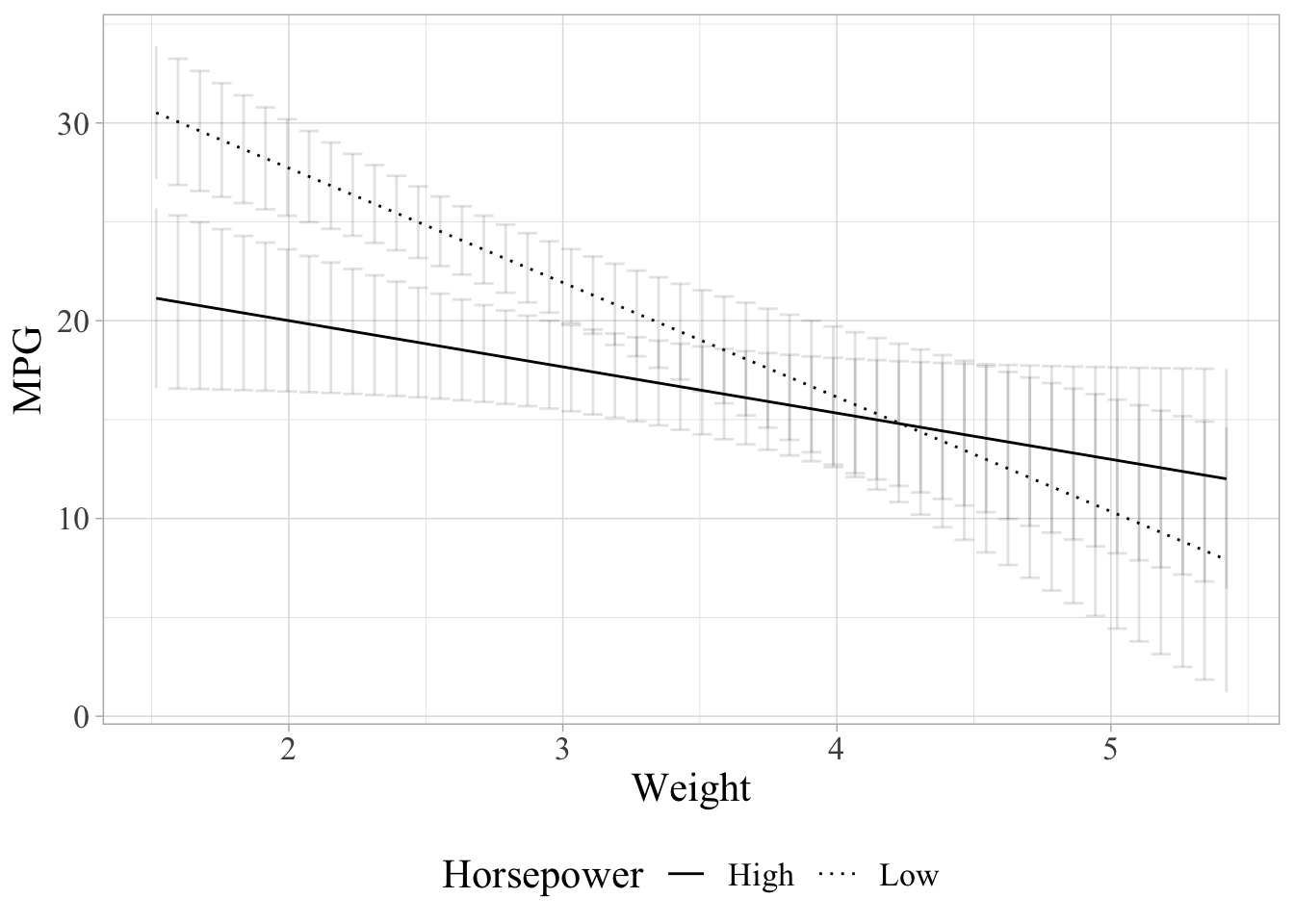

plot the moderating effect with a linear spline

library(lspline)
data(mtcars)
m3 <- lm(mpg ~ vs + carb + hp + lspline(wt, knots = 4, marginal = FALSE) * hp, data = mtcars)
plot_effect(reg.coef=summary(m3)$coefficients, data = mtcars, model = m3, 
            x_var.name = "wt", y_var.name = "mpg", moderator.name = "hp",
            xlab="Weight", ylab="MPG", moderator.lab="Horsepower") +
ggplot2::theme(text=ggplot2::element_text(family="Times New Roman", size = 16))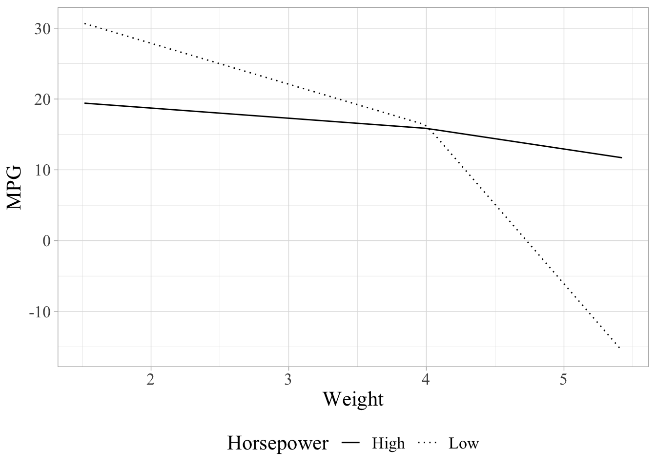

As we can see from the last line of code, the plot is customizable using “ggplot2”. There are a couple of other functions. Please see the reference manual on R documentation for details.

I’m also aiming to expand the package’s usage around its core functions. If you have any ideas or want to report a bug, please contact me or suggest on the GitHub page.

“regrrr”: One-stop R-toolkit for Compiling Regression Results

2019/03/06