DGP
set.seed(66)
# Generate Exogenous Variables
df <- data.frame(X = runif(300) * 10,
W = runif(300) * 5,
U = runif(300) * 2,
Z = c(rep(0, 150), rep(1, 150))) %>%
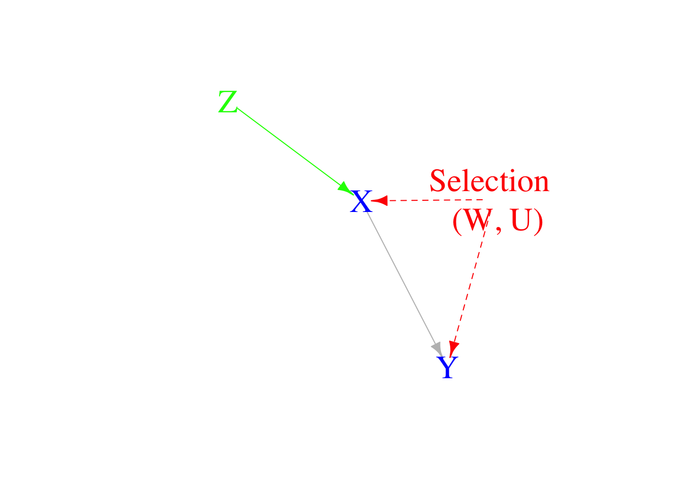
# God's Game
# X (Visible) affects Y, W (Invisible) and U (Invisible) affect Y
mutate(Y = .1 + .5*X + 0.8*W + 0.2*U + rnorm(300),
# X (Visible) affects Y, W (Invisible) and U (Invisible) affect Latent Selection Function
# Z (Visible) affect Latent Selection Function
select_ = 10 + 3*X + 2*W + 1*U + .5*Z + rnorm(300),
# Latent Selection Determines the True Selection
select = ifelse(select_ > mean(select_), 1, 0)
)
Run Heckman Regression
run_selection <- glm(select ~ X + Z, family = binomial( link = "probit" ), data = df)
df$IMR <- dnorm(run_selection$linear.predictors)/pnorm(run_selection$linear.predictors)
summary(run_selection)
##
## Call:
## glm(formula = select ~ X + Z, family = binomial(link = "probit"),
##     data = df)
##
## Deviance Residuals:
##     Min       1Q   Median       3Q      Max
## -2.0059  -0.1287  -0.0013   0.1240   2.5195
##
## Coefficients:
##             Estimate Std. Error z value Pr(>|z|)
## (Intercept)  -5.4514     0.6613  -8.244   <2e-16 ***
## X             1.0163     0.1213   8.380   <2e-16 ***
## Z             0.6183     0.2704   2.287   0.0222 *
## ---
## Signif. codes:  0 '***' 0.001 '**' 0.01 '*' 0.05 '.' 0.1 ' ' 1
##
## (Dispersion parameter for binomial family taken to be 1)
##
##     Null deviance: 415.03  on 299  degrees of freedom
## Residual deviance: 113.84  on 297  degrees of freedom
## AIC: 119.84
##
## Number of Fisher Scoring iterations: 8
run_outcome <- lm(Y ~ IMR + X, data = df[which(df$select == 1),])
summary(run_outcome)
##
## Call:
## lm(formula = Y ~ IMR + X, data = df[which(df$select == 1), ])
##
## Residuals:
##     Min      1Q  Median      3Q     Max
## -3.4067 -0.8600  0.0496  0.7680  3.4331
##
## Coefficients:
##             Estimate Std. Error t value Pr(>|t|)
## (Intercept)   2.4928     0.8875   2.809  0.00569 **
## IMR           0.9237     0.4398   2.100  0.03749 *
## X             0.4922     0.1099   4.477 1.56e-05 ***
## ---
## Signif. codes:  0 '***' 0.001 '**' 0.01 '*' 0.05 '.' 0.1 ' ' 1
##
## Residual standard error: 1.338 on 139 degrees of freedom
## Multiple R-squared:  0.1532, Adjusted R-squared:  0.141
## F-statistic: 12.58 on 2 and 139 DF,  p-value: 9.55e-06
Double Check
# Run OLS (which is biased)
run_biased <- lm(Y ~ X, data = df[which(df$select == 1),])
summary(run_biased)
##
## Call:
## lm(formula = Y ~ X, data = df[which(df$select == 1), ])
##
## Residuals:
##     Min      1Q  Median      3Q     Max
## -3.5643 -0.9695  0.1065  0.7926  3.2590
##
## Coefficients:
##             Estimate Std. Error t value Pr(>|t|)
## (Intercept)   4.0168     0.5172   7.766 1.55e-12 ***
## X             0.3114     0.0692   4.500 1.42e-05 ***
## ---
## Signif. codes:  0 '***' 0.001 '**' 0.01 '*' 0.05 '.' 0.1 ' ' 1
##
## Residual standard error: 1.354 on 140 degrees of freedom
## Multiple R-squared:  0.1263, Adjusted R-squared:  0.1201
## F-statistic: 20.25 on 1 and 140 DF,  p-value: 1.419e-05
# Check the Inclusion Restriction
run_test_instrument <- lm(Y ~ X + Z, data = df[which(df$select == 1),])
summary(run_test_instrument)
##
## Call:
## lm(formula = Y ~ X + Z, data = df[which(df$select == 1), ])
##
## Residuals:
##     Min      1Q  Median      3Q     Max
## -3.3369 -0.9958  0.1245  0.8445  3.1289
##
## Coefficients:
##             Estimate Std. Error t value Pr(>|t|)
## (Intercept)  3.71761    0.54715   6.794 2.93e-10 ***
## X            0.32192    0.06913   4.657 7.42e-06 ***
## Z            0.37117    0.23158   1.603    0.111
## ---
## Signif. codes:  0 '***' 0.001 '**' 0.01 '*' 0.05 '.' 0.1 ' ' 1
##
## Residual standard error: 1.347 on 139 degrees of freedom
## Multiple R-squared:  0.1422, Adjusted R-squared:  0.1299
## F-statistic: 11.52 on 2 and 139 DF,  p-value: 2.347e-05
# In Reality, Only God Can Run This Regression (by Knowing about the Truth and Seeing the Invisibles).
run_ture <- lm(Y ~ U + W + X, data = df)
summary(run_ture)
##
## Call:
## lm(formula = Y ~ U + W + X, data = df)
##
## Residuals:
##      Min       1Q   Median       3Q      Max
## -3.02525 -0.64811 -0.01175  0.56035  2.71664
##
## Coefficients:
##             Estimate Std. Error t value Pr(>|t|)
## (Intercept) 0.008025   0.188084   0.043  0.96600
## U           0.330793   0.099258   3.333  0.00097 ***
## W           0.773520   0.040014  19.331  < 2e-16 ***
## X           0.499843   0.020288  24.637  < 2e-16 ***
## ---
## Signif. codes:  0 '***' 0.001 '**' 0.01 '*' 0.05 '.' 0.1 ' ' 1
##
## Residual standard error: 0.9544 on 296 degrees of freedom
## Multiple R-squared:  0.7703, Adjusted R-squared:  0.768
## F-statistic: 330.9 on 3 and 296 DF,  p-value: < 2.2e-16